Longitudinal Continuous Outcomes in Clinical Trials: RM-ANOVA, LMM, MMRM and cLDA

Introduction

Continuous outcomes measured repeatedly over time are extremely common in clinical trials.

Examples include:

• blood pressure;
• body weight;
• bone mineral density;
• symptom scores;
• laboratory values;
• functional measures.

Several statistical approaches may appear suitable:

• mixed-design repeated-measures ANOVA;
• linear mixed-effects model;
• Mixed Model for Repeated Measures (MMRM);
• constrained longitudinal data analysis (cLDA).

These methods are related, but they are not interchangeable.

Learning objectives

By the end of this guide, the reader should be able to:

1. Explain the role and limitations of mixed-design RM-ANOVA.
2. Distinguish fixed and random effects in linear mixed models.
3. Explain how MMRM models repeated continuous outcomes in clinical trials.
4. Compare random-effects LMM with typical clinical-trial MMRM.
5. Describe the role of cLDA and baseline constraints.
6. Interpret covariance structures used in longitudinal models.

ANCOVA as the simplest baseline-adjusted model

Suppose a trial measures:

• baseline outcome $Y_0$;
• Week-24 outcome $Y_{24}$.

A common model is:

$$Y_{24} = \beta_0+ \beta_1Treatment+ \beta_2Y_0+ \epsilon$$

Here, $\beta_1$ estimates the baseline-adjusted treatment-group difference.

This is often preferable to analysing only:

$$Y_{24}-Y_0$$

because ANCOVA explicitly models the relationship between baseline and follow-up outcome.[1]

Mixed-design repeated-measures ANOVA

Suppose outcomes are measured at baseline, Week 4, Week 8 and Week 12.

A simplified model is:

$$Y_{ij} = \mu+ Treatment_i+ Time_j+ Treatment_i\times Time_j+ \epsilon_{ij}$$

Treatment is a between-subject factor and time is a within-subject factor.

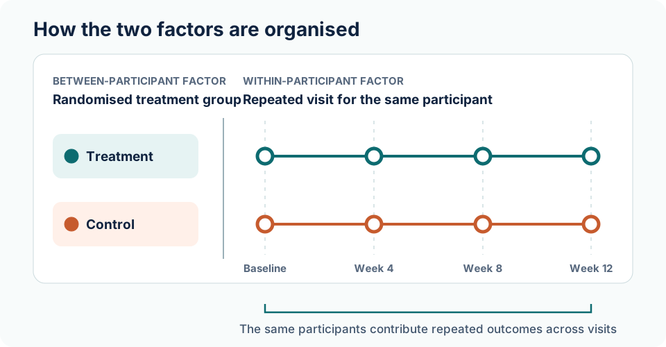
The main effects are:

• treatment;
• time;
• treatment × time.

The interaction asks whether the treatment groups follow different patterns over time.

Why RM-ANOVA is often not the modern default

Traditional RM-ANOVA can be restrictive when there are:[2]

• missing observations;
• unequal follow-up;
• complex covariance patterns;
• irregular timing;
• multilevel clustering.

It also commonly relies on assumptions concerning the covariance of repeated measurements, including sphericity.

When sphericity is violated, corrections such as:

• Greenhouse-Geisser;
• Huynh-Feldt;

may be used.

These corrections adjust degrees of freedom. They do not solve the broader problems of missing data, estimands or complex longitudinal structure.

Linear mixed-effects models

A general linear mixed model is:

$$Y=X\beta+Zb+\epsilon$$

where:

• $X\beta$ represents fixed effects;
• $Zb$ represents random effects;
• $\epsilon$ represents residual variation.

Random intercept model

A random-intercept model may be written as:

$$Y_{ij} = \beta_0+ \beta_1Treatment_i+ \beta_2Time_{ij} + b_{0i} + \epsilon_{ij}$$

with:

$$b_{0i}\sim N(0,\sigma_b^2)$$

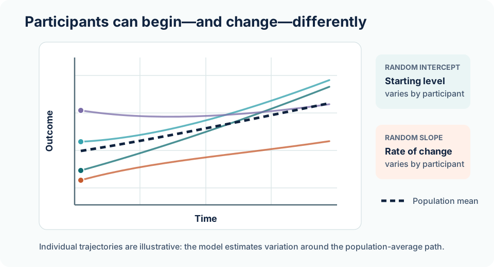
Each participant has an individual intercept that deviates from the population intercept.

Random slope model

Participants may also differ in rate of change:

$$Y_{ij} = \beta_0+ \beta_1Treatment_i+ \beta_2Time_{ij} + b_{0i} + b_{1i}Time_{ij} + \epsilon_{ij}$$

This allows:

• participant-specific starting levels;
• participant-specific trajectories.

Why LMM is powerful

LMMs can represent correlation generated by:

• repeated measurements within participants;
• patients within hospitals;
• repeated observations within clinicians;
• multilevel structures.

For example:

$$Measurement \subset Patient \subset Centre$$

The strength of the LMM is therefore its ability to model hierarchy and dependence, not merely its ability to retain incomplete cases.

Mixed Model for Repeated Measures

MMRM is widely used for scheduled repeated continuous outcomes in clinical trials.

A typical model may include:

$$Y_{ij} = Treatment_i + Visit_j + Treatment_i\times Visit_j + Baseline_i + Baseline_i\times Visit_j + \epsilon_{ij}$$

Repeated residuals within participant are assumed to follow a covariance matrix:

$$\epsilon_i\sim N(0,\Sigma)$$

MMRM commonly:

• treats visit as categorical;
• includes treatment × visit;
• adjusts for baseline;
• directly models within-participant covariance;
• does not necessarily include random slopes.

Why visit is often categorical

If time is modelled as a single continuous variable:

$$Y=\beta_0+\beta_1Time$$

the model imposes a functional form.

Treating visit as categorical allows each visit to have its own mean.

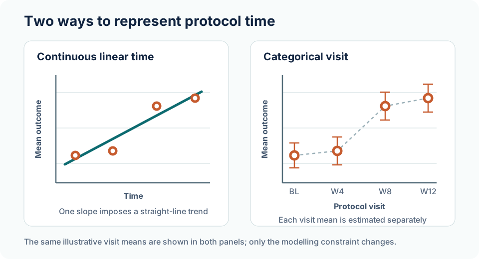
This is useful when the treatment effect at specific protocol-defined visits is important.

Treatment-by-visit interaction

With treatment × visit included:

$$\Delta_4 \neq \Delta_8 \neq \Delta_{12}$$

where:

$$\Delta_j = \mu_{Treatment,j} - \mu_{Control,j}$$

If the primary estimand concerns Week 24, the main contrast may be:

$$\Delta_{24}$$

even though earlier visits contribute to the longitudinal model.

Covariance structures

Compound symmetry

All pairs of visits have the same correlation:

$$R= \begin{pmatrix} 1&\rho&\rho\\ \rho&1&\rho\\ \rho&\rho&1 \end{pmatrix}$$

AR(1)

Correlation decays with visit separation:

$$Corr(Y_j,Y_k) = \rho^{|j-k|}$$

Toeplitz

Correlation depends on lag but does not need to follow geometric decay.

Unstructured

Each variance and covariance is separately estimated:

$$\Sigma= \begin{pmatrix} \sigma_1^2 & \sigma_{12} & \sigma_{13}\\ \sigma_{12} & \sigma_2^2 & \sigma_{23}\\ \sigma_{13} & \sigma_{23} & \sigma_3^2 \end{pmatrix}$$

For $k$ visits, an unstructured covariance matrix estimates:

$$\frac{k(k+1)}{2}$$

parameters.

MMRM versus random-effects LMM

These are common practical distinctions rather than strict mathematical boundaries.

Estimated marginal means

Suppose:

$$\hat{\mu}_{Treatment,24}$$

and:

$$\hat{\mu}_{Control,24}$$

are model-based estimated marginal means at Week 24.

Then:

$$\hat{\Delta}_{24} = \hat{\mu}_{Treatment,24} - \hat{\mu}_{Control,24}$$

A good report should present:

• estimated treatment difference;
• 95% confidence interval;
• units;
• direction of benefit;
• prespecified p-value where relevant.

Constrained longitudinal data analysis

cLDA includes baseline within the longitudinal outcome vector:

$$Y_i= \begin{pmatrix} Y_{Baseline}\\ Y_{Week12}\\ Y_{Week24} \end{pmatrix}$$

Because treatment is randomised after baseline, cLDA commonly constrains baseline population means to equality:[3][4]

$$\mu_{Treatment,Baseline} = \mu_{Control,Baseline}$$

Degrees of freedom

Mixed-model inference may use finite-sample approximations such as:

• Satterthwaite;
• Kenward-Roger.

These become particularly relevant with:

• modest sample size;
• complex covariance structures;
• unequal group sizes;
• incomplete repeated observations.

Clinical example

Suppose:

• 140 participants;
• two treatment groups;
• continuous functional score;
• measurements at baseline, Week 4, Week 12 and Week 24;
• primary question: treatment difference at Week 24.

Possible approaches include:

ANCOVA

Uses Week-24 outcome and baseline adjustment.

RM-ANOVA

Uses repeated outcomes but may focus on a global interaction and restrictive covariance assumptions.

MMRM

Uses all scheduled post-baseline observations and directly estimates the Week-24 marginal treatment contrast.

Random-effects LMM

May be attractive if individual trajectories or slopes are scientifically important.

cLDA

Models baseline and follow-up jointly with equal baseline means constrained.

Common mistakes

”MMRM is simply RM-ANOVA with missing data”

Incorrect. MMRM belongs to the mixed-model framework and offers more flexible covariance modelling and likelihood-based estimation.

”Use unstructured covariance because it is most flexible”

Flexibility comes at the cost of many parameters and possible instability.

”Choose the covariance structure that gives the smallest p-value”

Confirmatory analyses should be prespecified or based on defensible prespecified selection rules.

”A significant treatment × time interaction proves benefit at the target visit”

Not necessarily. The primary contrast may be the treatment difference at a specific visit.

Practical checklist

• Is the primary treatment contrast visit-specific or trajectory-based?
• Is time better treated as categorical or continuous?
• Is baseline included appropriately?
• Is a random intercept or slope scientifically meaningful?
• Is the covariance structure defensible?
• Are degrees-of-freedom adjustments prespecified?
• Are missing-data assumptions explicit?
• Does the model estimate the intended estimand?

Key takeaways

1. RM-ANOVA is useful historically and pedagogically but is often restrictive for modern clinical trials.
2. LMM provides a broad framework for continuous correlated and hierarchical data.
3. MMRM is especially useful for scheduled repeated continuous efficacy outcomes with visit-specific treatment contrasts.
4. cLDA provides an alternative longitudinal formulation that includes baseline as part of the response.
5. Covariance structure is a substantive modelling decision, not a software setting to select mechanically.

References

1. US Food and Drug Administration. Adjusting for Covariates in Randomized Clinical Trials for Drugs and Biological Products: Guidance for Industry. 2023. Available from: https://www.fda.gov/regulatory-information/search-fda-guidance-documents/adjusting-covariates-randomized-clinical-trials-drugs-and-biological-products

2. Gueorguieva R, Krystal JH. Move over ANOVA: progress in analyzing repeated-measures data and its reflection in papers published in the Archives of General Psychiatry. Arch Gen Psychiatry. 2004;61(3):310-317. doi:10.1001/archpsyc.61.3.310

3. Liu GF, Lu K, Mogg R, Mallick M, Mehrotra DV. Should baseline be a covariate or dependent variable in analyses of change from baseline in clinical trials? Stat Med. 2009;28(20):2509-2530. doi:10.1002/sim.3639

4. Lu K. On efficiency of constrained longitudinal data analysis versus longitudinal analysis of covariance. Biometrics. 2010;66(3):891-896. doi:10.1111/j.1541-0420.2009.01332.x